Come si fa a sommare i valori compresi tra due date in Excel?
Quando nel foglio di lavoro sono presenti due elenchi, come illustrato nello screenshot a destra — uno con le date e l’altro con i valori — e si desidera sommare solo i valori compresi tra due date specifiche, ad esempio dal 3/4/2014 al 5/10/2014, come si può effettuare il calcolo in modo rapido? Di seguito è riportata una formula per sommarli direttamente in Excel.
- Somma valori compresi tra due date con una formula in Excel
- Somma valori compresi tra due date con un filtro in Excel
Somma valori compresi tra due date con una formula in Excel
Fortunatamente, esiste una formula in grado di sommare i valori compresi tra due date in Excel.
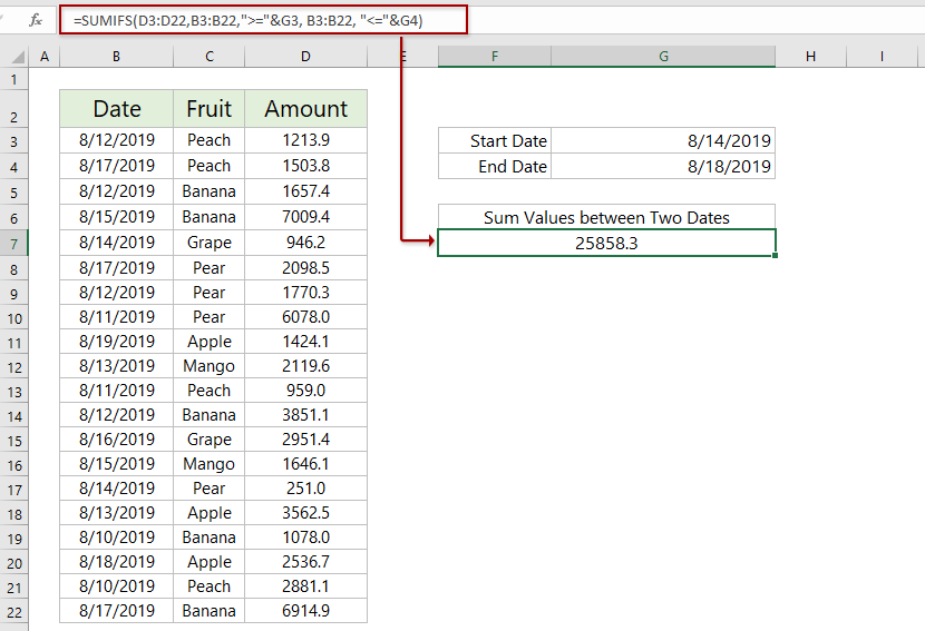
Seleziona una cella vuota, digita la formula seguente e premi Invio. Otterrai immediatamente il risultato del calcolo. Guarda lo screenshot:
=SUMIFS(B2:B8,A2:A8,">="&E2,A2:A8,"<="&E3)
Nota: Nella formula precedente,
- D3:D22è l'elenco dei valori che sommerai
- B3:B22è l'elenco delle date in base al quale effettuerai la somma
- G3è la cella con Data di inizio
- G4è la cella con Data di fine
 | La formula è troppo complicata da ricordare? Salvatala come voce di Testo automatico e riutilizzala in futuro con un solo clic!Ulteriori informazioni… Prova gratuita |
Somma facilmente i dati per ogni Anno fiscale, ogni Semestre o ogni settimana in Excel
La funzione **Raggruppamento temporale speciale** di Kutools per Excel ti permette di aggiungere una colonna helper per calcolare automaticamente l’**Anno fiscale**, il **Semestre**, il **Numero di settimana** o il **Giorno della settimana** in base a una colonna Data specifica, e di contare, sommare o calcolare la media dei valori in base a questi raggruppamenti direttamente in una nuova Tabella pivot.
Kutools per Excel– Potenzia Excel con oltre 300 strumenti essenziali, rendendo il tuo lavoro più veloce e semplice, e sfrutta le funzionalità basate sull’IA per un’elaborazione dati più intelligente e una maggiore produttività.Scaricalo ora
Somma valori compresi tra due date con un filtro in Excel
Se devi sommare valori compresi tra due date e l’intervallo di date cambia frequentemente, puoi aggiungere un gruppo per quell’intervallo specifico e utilizzare quindi la funzione SUBTOTALE per sommare i valori nell’intervallo di date desiderato in Excel.
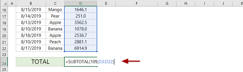
1. Seleziona una cella vuota, inserisci la formula seguente e premi Invio.
=SUBTOTALE(109;D3:D22)
Nota: nella formula precedente, 109 indica la somma dei valori filtrati; D3:D22 rappresenta l’intervallo di valori da sommare.
2. Seleziona l'intestazione dell'intervallo e applica il filtro facendo clic su Dati > Filtro.
3. Fai clic sull'icona del filtro nell'intestazione della colonna Data e seleziona Filtri data > Compreso tra. Nella finestra di dialogo Filtro automatico personalizzato, inserisci la data di inizio e la data di fine desiderate, quindi fai clic sul pulsante OK. Il valore totale verrà aggiornato automaticamente in base ai dati filtrati.
Articoli correlati:
Migliori Strumenti per la Produttività in Office
Potenzia le tue competenze in Excel con Kutools per Excel e sperimenta un’efficienza mai vista prima.Kutools per Excel offre oltre 300 funzionalità avanzate per aumentare la produttività e Risparmia tempo.Clicca qui per ottenere la funzionalità di cui hai più bisogno...
Office Tab Porta l'interfaccia a schede in Office e rende il tuo lavoro molto più semplice
- Abilita la modifica e la lettura a schede in Word, Excel, PowerPoint, Publisher, Access, Visio e Project.
- Apri e crea più documenti in nuove schede all’interno della stessa finestra, invece che in finestre separate.
- Aumenta la tua produttività del 50 % e risparmia centinaia di clic del mouse ogni giorno!
Tutti i componenti aggiuntivi di Kutools in un unico programma di installazione.
Kutools for Office è la suite che include componenti aggiuntivi per Excel, Word, Outlook e PowerPoint, oltre a Office Tab Pro: la soluzione ideale per i team che lavorano su diverse app di Office.
- Suite completa— componenti aggiuntivi per Excel, Word, Outlook e PowerPoint + Office Tab Pro
- Un unico programma di installazione, una sola licenza— configurazione in pochi minuti (pronto per MSI)
- Funziona meglio insieme— produttività ottimizzata tra le app di Office
- Prova gratuita di 30 giorni con tutte le funzionalità— nessuna registrazione, nessuna carta di credito
- Miglior rapporto qualità-prezzo— risparmia rispetto all’acquisto dei singoli componenti aggiuntivi