Come trovare il primo o l’ultimo venerdì di ogni mese in Excel?
Di norma, il venerdì è l’ultimo giorno lavorativo del mese. Ma come individuare il primo o l’ultimo venerdì a partire da una data specifica in Excel? In questo articolo ti guideremo passo dopo passo nell’utilizzo di due formule semplici ed efficaci per trovare il primo e l’ultimo venerdì di ogni mese.
Trovare il primo venerdì di un mese
Trovare l’ultimo venerdì di un mese
Trovare il primo venerdì di un mese
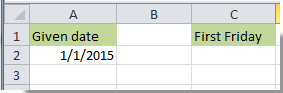
Ad esempio, la data specificata (1/1/2015) si trova nella cella A2, come illustrato nello screenshot seguente. Per trovare il primo venerdì del mese in base alla data indicata, procedi nel modo seguente.
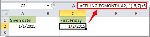
1. Seleziona la cella in cui desideri visualizzare il risultato; in questo caso, scegliamo la cella C2.
2. Copia e incolla la formula seguente al suo interno, quindi premi Invio.
=CEILING(EOMONTH(A2,-1)-5,7)+6
Note:
Trovare l’ultimo venerdì di un mese
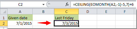
La data specificata, 1/1/2015, si trova nella cella A2; per trovare l’ultimo venerdì di quel mese in Excel, procedi come segue.
1. Seleziona una cella, incolla la formula seguente al suo interno e premi Invio per ottenere il risultato.
=DATE(YEAR(A2),MONTH(A2)+1,0)+MOD(-WEEKDAY(DATE(YEAR(A2),MONTH(A2)+1,0),2)-2,-7)

Nota: Puoi sostituire A2 nella formula con il riferimento alla cella che contiene la data specificata.
Articoli correlati:
- Come trovare i 5 valori più bassi e i 5 valori più alti in un elenco in Excel?
- Come verificare se una determinata cartella di lavoro è aperta in Excel?
- Come si fa a capire se una cella è referenziata in un’altra cella in Excel?
- Come trovare la data più vicina a oggi in un elenco di Excel?
Migliori Strumenti per la Produttività in Office
Potenzia le tue competenze in Excel con Kutools per Excel e sperimenta un’efficienza mai vista prima.Kutools per Excel offre oltre 300 funzionalità avanzate per aumentare la produttività e Risparmia tempo.Clicca qui per ottenere la funzionalità di cui hai più bisogno...
Office Tab Porta l'interfaccia a schede in Office e rende il tuo lavoro molto più semplice
- Abilita la modifica e la lettura a schede in Word, Excel, PowerPoint, Publisher, Access, Visio e Project.
- Apri e crea più documenti in nuove schede all’interno della stessa finestra, invece che in finestre separate.
- Aumenta la tua produttività del 50 % e risparmia centinaia di clic del mouse ogni giorno!
Tutti i componenti aggiuntivi di Kutools in un unico programma di installazione.
Kutools for Office è la suite che include componenti aggiuntivi per Excel, Word, Outlook e PowerPoint, oltre a Office Tab Pro: la soluzione ideale per i team che lavorano su diverse app di Office.
- Suite completa— componenti aggiuntivi per Excel, Word, Outlook e PowerPoint + Office Tab Pro
- Un unico programma di installazione, una sola licenza— configurazione in pochi minuti (pronto per MSI)
- Funziona meglio insieme— produttività ottimizzata tra le app di Office
- Prova gratuita di 30 giorni con tutte le funzionalità— nessuna registrazione, nessuna carta di credito
- Miglior rapporto qualità-prezzo— risparmia rispetto all’acquisto dei singoli componenti aggiuntivi