Come usare CERCA.VERT per restituire più valori in un’unica cella in Excel?
CERCA.VERT è una funzione potente in Excel, ma per impostazione predefinita restituisce solo il primo valore corrispondente. E se avessi bisogno di recuperare **tutti** i valori corrispondenti e combinarli in un’unica cella? È un’esigenza comune quando si analizzano set di dati o si sintetizzano informazioni. In questa guida ti mostreremo passo dopo passo diversi metodi per restituire più valori in un’unica cella, sfruttando sia formule avanzate che funzionalità integrate di Excel.
Restituisci più valori in un’unica cella con la funzione TESTO.CONCAT (Excel 2019 e Office 365)
- Restituisci tutti i valori corrispondenti in un’unica cella
- Restituisci tutti i valori corrispondenti senza duplicati in un’unica cella
Restituisci più valori in un’unica cella con Kutools
Restituisci più valori in un’unica cella con una funzione definita dall’utente
- Restituisci tutti i valori corrispondenti in un’unica cella
- Restituisci tutti i valori corrispondenti senza duplicati in un’unica cella
Restituisci più valori in un’unica cella con la funzione TESTO.CONCAT (Excel 2019 e Office 365)
Se hai una versione più recente di Excel, come Excel 2019 o Office 365, puoi sfruttare una nuova funzione – TEXTJOIN – che ti permette di usare rapidamente CERCA.VERT per restituire tutti i valori corrispondenti in un’unica cella.
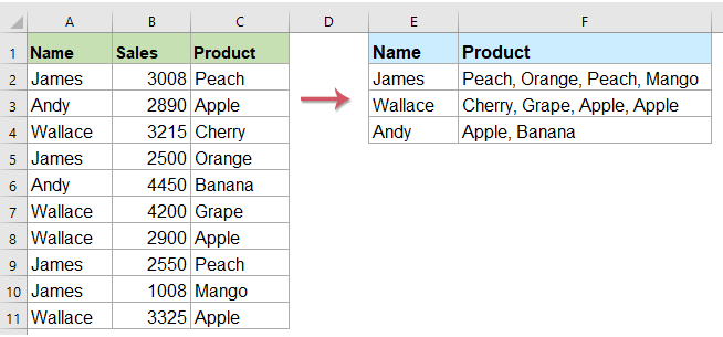
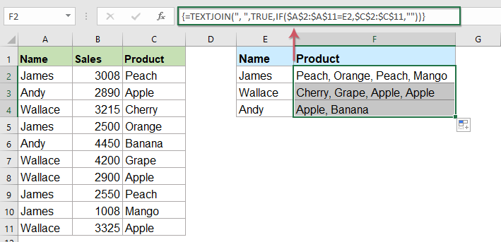
Restituisci tutti i valori corrispondenti in un’unica cella
Applica la formula seguente in una cella vuota in cui desideri visualizzare il risultato, premi contemporaneamente Ctrl + Maiusc + Invio per ottenere il primo risultato, quindi trascina il quadratino di riempimento verso il basso fino alla cella in cui vuoi applicare la formula: otterrai così tutti i valori corrispondenti, come mostrato nell’immagine seguente:
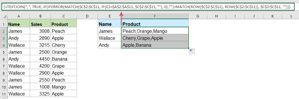
Restituisci tutti i valori corrispondenti senza duplicati in un’unica cella
Se desideri ottenere tutti i valori corrispondenti in base ai criteri di ricerca, senza duplicati, la seguente formula potrebbe fare al caso tuo.
Copia e incolla la formula seguente in una cella vuota, premi contemporaneamente Ctrl + Maiusc + Invio per ottenere il primo risultato, quindi copia la formula nelle altre celle: otterrai tutti i valori corrispondenti senza duplicati, come mostrato nell’immagine seguente:
Restituisci più valori in un’unica cella con Kutools
Grazie alla funzione «Unione avanzata righe» di Kutools per Excel, puoi recuperare facilmente più valori corrispondenti in un’unica cella, senza dover ricorrere a formule complesse! Dì addio ai metodi manuali e scopri un modo più efficiente per gestire le tue ricerche in Excel. Scopriamo insieme come Kutools per Excel rende tutto questo possibile!
Dopo aver installato Kutools per Excel, procedi come segue:
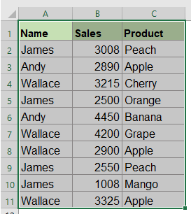
1. Seleziona l’intervallo di dati in base al quale desideri combinare i dati di una colonna.
2. Fai clic su «Kutools» > «Unisci e Dividi» > «Unione avanzata righe», come mostrato nello screenshot:

3. Nella finestra di dialogo visualizzata, «Unione avanzata righe»:
- Fai clic sul nome della colonna chiave in base alla quale combinare i dati, quindi seleziona «Chiave primaria».
- Quindi fai clic su un’altra colonna i cui dati desideri combinare in base alla colonna chiave, apri l’elenco a discesa nel campo «Operazione» e seleziona un separatore per dividere i dati combinati nella sezione «Combina».
- Quindi, fai clic sul pulsante OK.

Tutti i valori corrispondenti provenienti da un’altra colonna, associati allo stesso valore, vengono combinati in un’unica cella. Vedi screenshot:
 |  |
Suggerimenti: se desideri eliminare i contenuti duplicati durante l’unione delle celle, basta selezionare l’opzione «Elimina valori duplicati» nella finestra di dialogo. In questo modo verranno combinati solo i valori univoci, rendendo i tuoi dati più puliti e organizzati senza alcuno sforzo aggiuntivo. Vedi screenshot:
 |  |
Scarica subito la versione di prova gratuita di Kutools per Excel!
Restituisci più valori in un’unica cella con una funzione definita dall’utente
La funzione TESTO.CONCAT descritta sopra è disponibile esclusivamente in Excel 2019 e Office 365; se utilizzi versioni precedenti di Excel, devi ricorrere a codici specifici per eseguire questa operazione.
Restituisci tutti i valori corrispondenti in un’unica cella
1. Tieni premuti i tasti «ALT + F11» per aprire la finestra di Microsoft Visual Basic, Applications.
2. Fai clic su «Inserisci» > «Modulo» e incolla il codice seguente nella finestra del modulo.
Codice VBA: CERCA.VERT per restituire più valori in un’unica cella
Function ConcatenateIf(CriteriaRange As Range, Condition As Variant, ConcatenateRange As Range, Optional Separator As String = ",") As Variant
'Updateby Extendoffice
Dim xResult As String
On Error Resume Next
If CriteriaRange.Count <> ConcatenateRange.Count Then
    ConcatenateIf = CVErr(xlErrRef)
    Exit Function
End If
For i = 1 To CriteriaRange.Count
    If CriteriaRange.Cells(i).Value = Condition Then
        xResult = xResult & Separator & ConcatenateRange.Cells(i).Value
    End If
Next i
If xResult <> "" Then
    xResult = VBA.Mid(xResult, VBA.Len(Separator) + 1)
End If
ConcatenateIf = xResult
Exit Function
End Function
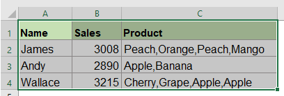
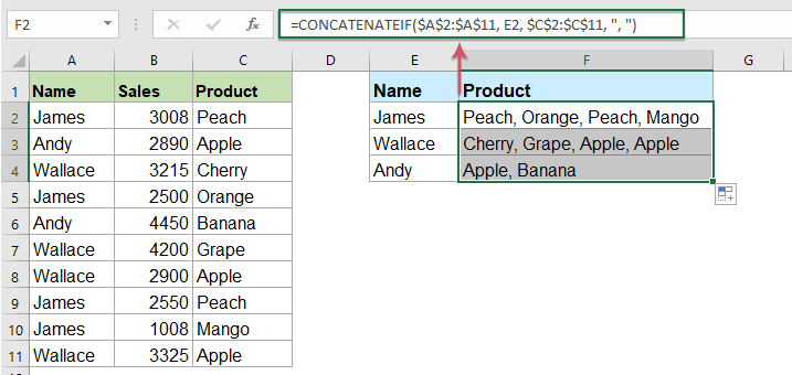
3. Salva e chiudi quindi questo codice, torna al foglio di lavoro e inserisci la seguente formula: =CONCATENATEIF($A$2:$A$11, E2, $C$2:$C$11, ", ") in una cella vuota a tua scelta per visualizzare il risultato; infine, trascina il quadratino di riempimento verso il basso per ottenere tutti i valori corrispondenti in un’unica cella, come mostrato nello screenshot:
Restituisci tutti i valori corrispondenti senza duplicati in un’unica cella
Per ignorare i duplicati tra i valori corrispondenti restituiti, utilizza il codice seguente.
1. Tieni premuti i tasti «Alt + F11» per aprire la finestra di Microsoft Visual Basic, Applications.
2. Fai clic su «Inserisci» > «Modulo» e incolla il codice seguente nella finestra del modulo.
Codice VBA: CERCA.VERT e restituzione di più valori univoci corrispondenti in un’unica cella
Function MultipleLookupNoRept(Lookupvalue As String, LookupRange As Range, ColumnNumber As Integer)
'Updateby Extendoffice
    Dim xDic As New Dictionary
    Dim xRows As Long
    Dim xStr As String
    Dim i As Long
    On Error Resume Next
    xRows = LookupRange.Rows.Count
    For i = 1 To xRows
        If LookupRange.Columns(1).Cells(i).Value = Lookupvalue Then
            xDic.Add LookupRange.Columns(ColumnNumber).Cells(i).Value, ""
        End If
    Next
    xStr = ""
    MultipleLookupNoRept = xStr
    If xDic.Count > 0 Then
        For i = 0 To xDic.Count - 1
            xStr = xStr & xDic.Keys(i) & ","
        Next
        MultipleLookupNoRept = Left(xStr, Len(xStr) - 1)
    End If
End Function
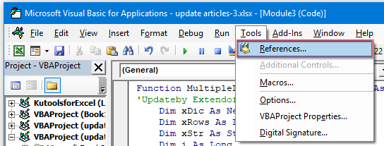
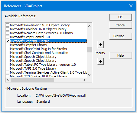
3. Dopo aver inserito il codice, fai clic su **Strumenti** > **Riferimenti** nella finestra di **Microsoft Visual Basic, Applications** che si è aperta; nella finestra di dialogo **Riferimenti – VBAProject** visualizzata, seleziona l’opzione **Microsoft Scripting Runtime** nell’elenco **Riferimenti disponibili** (vedi screenshot):
 |  |
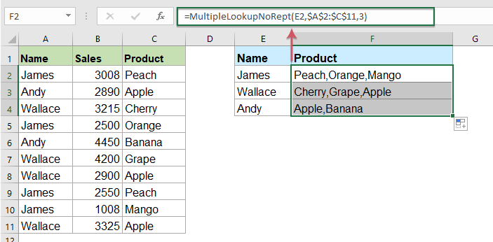
4. Fai quindi clic su OK per chiudere la finestra di dialogo, salva e chiudi la finestra del codice, torna al foglio di lavoro e inserisci la seguente formula: =MultipleLookupNoRept(E2,$A$2:$C$11,3) in una cella vuota dove desideri visualizzare il risultato; infine, trascina il quadratino di riempimento verso il basso per ottenere tutti i valori corrispondenti, come mostrato nello screenshot:
Che tu scelga formule come TESTO.CONCAT abbinate a funzioni matriciali, strumenti come
Altri articoli correlati:
- Funzione CERCA.VERT con alcuni esempi di base e avanzati
- In Excel, la funzione CERCA.VERT è uno strumento potente per la maggior parte degli utenti: cerca un valore nella colonna più a sinistra di un intervallo di dati e restituisce il valore corrispondente nella stessa riga da una colonna specificata. Questo tutorial mostra come utilizzare la funzione CERCA.VERT con esempi sia base che avanzati in Excel.
- Restituisci più valori corrispondenti in base a uno o più criteri
- Di solito, trovare un valore specifico e restituire l’elemento corrispondente è semplice per la maggior parte di noi grazie alla funzione CERCA.VERT. Ma hai mai provato a restituire più valori corrispondenti in base a uno o più criteri? In questo articolo ti presenterò alcune formule efficaci per affrontare questa sfida complessa in Excel.
- CERCA.VERT e restituzione di più valori in verticale
- Normalmente, puoi usare la funzione CERCA.VERT per ottenere il primo valore corrispondente, ma a volte potresti voler restituire tutti i record corrispondenti in base a un criterio specifico. In questo articolo spiegherò come effettuare una ricerca con CERCA.VERT e restituire tutti i valori corrispondenti in verticale, in orizzontale o in un’unica cella.
- CERCA.VERT e restituzione di più valori da un elenco a discesa
- In Excel, come si può utilizzare CERCA.VERT per restituire più valori corrispondenti da un elenco a discesa, ovvero visualizzare immediatamente tutti i valori relativi quando si seleziona un elemento dall’elenco? In questo articolo presenterò la soluzione passo dopo passo.
Migliori Strumenti per la Produttività in Office
Potenzia le tue competenze in Excel con Kutools per Excel e sperimenta un’efficienza mai vista prima.Kutools per Excel offre oltre 300 funzionalità avanzate per aumentare la produttività e Risparmia tempo.Clicca qui per ottenere la funzionalità di cui hai più bisogno...
Office Tab Porta l'interfaccia a schede in Office e rende il tuo lavoro molto più semplice
- Abilita la modifica e la lettura a schede in Word, Excel, PowerPoint, Publisher, Access, Visio e Project.
- Apri e crea più documenti in nuove schede all’interno della stessa finestra, invece che in finestre separate.
- Aumenta la tua produttività del 50 % e risparmia centinaia di clic del mouse ogni giorno!
Tutti i componenti aggiuntivi di Kutools in un unico programma di installazione.
Kutools for Office è la suite che include componenti aggiuntivi per Excel, Word, Outlook e PowerPoint, oltre a Office Tab Pro: la soluzione ideale per i team che lavorano su diverse app di Office.
- Suite completa— componenti aggiuntivi per Excel, Word, Outlook e PowerPoint + Office Tab Pro
- Un unico programma di installazione, una sola licenza— configurazione in pochi minuti (pronto per MSI)
- Funziona meglio insieme— produttività ottimizzata tra le app di Office
- Prova gratuita di 30 giorni con tutte le funzionalità— nessuna registrazione, nessuna carta di credito
- Miglior rapporto qualità-prezzo— risparmia rispetto all’acquisto dei singoli componenti aggiuntivi