Estrai valori univoci in base a uno o più criteri in Excel
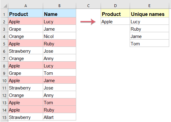
Estrarre valori univoci in base a criteri è un’operazione fondamentale per l’analisi dei dati e il reporting. Immagina di avere l’intervallo di dati a sinistra e di voler elencare solo i nomi univoci presenti nella colonna B, filtrati in base a un criterio specifico nella colonna A. Che tu stia utilizzando versioni più datate di Excel o le funzionalità avanzate di Excel 365/2021, questa guida ti mostrerà come estrarre valori univoci in modo rapido ed efficiente.
Estrai valori univoci in base a criteri in Excel
- Con formula matriciale
- Con Kutools per Excel
- Con formula (Excel 365, Excel 2021 e versioni successive)
Estrai valori univoci in base a criteri multipli in Excel
Estrai valori univoci da un elenco di celle con Kutools per Excel
Estrai valori univoci in base a criteri in Excel
•Con formula matriciale per elencare i valori univoci in verticale
Per risolvere questo compito, puoi utilizzare una formula matriciale avanzata. Procedi nel modo seguente:
1. Inserisci la seguente formula in una cella vuota dove desideri visualizzare il risultato estratto. In questo esempio, la inseriremo nella cella E2: premi quindi Maiusc + Ctrl + Invio per ottenere il primo valore univoco.
=IFERROR(INDEX($B$2:$B$15, MATCH(0, IF($D$2=$A$2:$A$15, COUNTIF($E$1:$E1, $B$2:$B$15), ""), 0)),"")2. Trascina quindi il quadratino di riempimento verso il basso finché non compaiono celle vuote. A questo punto, tutti i valori univoci in base al criterio specificato sono stati elencati; vedi screenshot:

•Estrai e visualizza valori univoci in un’unica cella utilizzando Kutools per Excel
Kutools per Excel ti offre un metodo semplice per estrarre valori univoci e visualizzarli in un’unica cella, risparmiandoti tempo e fatica quando lavori con set di dati di grandi dimensioni, senza dover ricordare alcuna formula.
Dopo aver installato Kutools per Excel, procedi come segue:
Fai clic su «Kutools» > «Super RICERCA.VERT» > «Ricerca uno-a-molti (restituisce più risultati)» per aprire la finestra di dialogo. Nella finestra visualizzata, configura le operazioni come indicato di seguito:
- Seleziona separatamente «Area di posizionamento dell'elenco» e «Intervallo di valore di ricerca» nei riquadri di testo;
- Seleziona l’intervallo della tabella che desideri utilizzare;
- Specifica separatamente Colonna chiave e Colonna di restituzione nei menu a discesa «Colonna chiave» e «Colonna di restituzione»;
- Infine, fai clic sul pulsante OK.


Risultato:
Tutti i nomi univoci in base al criterio sono stati estratti in un’unica cella, vedi screenshot:
•Con formula in Excel 365, Excel 2021 e versioni successive per elencare valori univoci in verticale
Con Excel 365 e Excel 2021, funzioni come UNIQUE e FILTER semplificano notevolmente l’estrazione di valori univoci.
Inserisci la seguente formula in una cella vuota e premi Invio per ottenere immediatamente tutti i nomi univoci in verticale.
=UNIQUE(FILTER(B2:B15, A2:A15=D2))
- FILTER(B2:B15, A2:A15=D2):
- FILTERFiltra i dati nell'intervallo B2:B15.
- A2:A15=D2Verifica dove i valori nell'intervallo A2:A15 corrispondono al valore in D2; solo le righe che soddisfano questa condizione vengono incluse nel risultato.
- UNIQUE(...):
garantisce che dai risultati filtrati vengano restituiti solo valori univoci.
Estrai valori univoci in base a criteri multipli in Excel
•Con formula matriciale per elencare i valori univoci in verticale
Se desideri estrarre valori univoci in base a due condizioni, ecco un’altra formula matriciale che fa al caso tuo. Procedi come segue:
1. Inserisci la seguente formula in una cella vuota dove desideri visualizzare i valori univoci. In questo esempio, la inseriremo nella cella G2: premi quindi Maiusc + Ctrl + Invio per ottenere il primo valore univoco.
=IFERROR(INDEX($C$2:$C$15,MATCH(0,COUNTIF(G1:$G$1,$C$2:$C$15)+IF($A$2:$A$15<>$E$2,1,0)+IF($B$2:$B$15<>$F$2,1,0),0)),"")2. Trascina quindi il quadratino di riempimento verso il basso finché non compaiono celle vuote. A questo punto, tutti i valori univoci corrispondenti alle due condizioni specifiche sono stati elencati, come mostrato nello screenshot:

•Con in Excel 365, Excel 2021 e versioni successive per elencare valori univoci in verticale
Con le versioni più recenti di Excel, estrarre valori univoci in base a criteri multipli è diventato molto più semplice.
Inserisci la seguente formula in una cella vuota e premi Invio per ottenere immediatamente tutti i nomi univoci in verticale.
=UNIQUE(FILTER(C2:C15, (A2:A15=E2) * (B2:B15=F2)))
- FILTER(C2:C15, (A2:A15=E2) * (B2:B15=F2)):
- FILTERFiltra i dati nell'intervallo C2:C15.
- (A2:A15=E2)Verifica se i valori nella colonna A corrispondono al valore presente in E2.
- (B2:B15=F2)Verifica se i valori nella colonna B corrispondono al valore presente in F2.
- *: combina le due condizioni con la logica AND, il che significa che entrambe devono essere vere affinché una riga venga inclusa.
- UNIQUE(...):
Rimuove i valori duplicati dai risultati filtrati, assicurando che l’output includa esclusivamente valori univoci.
Estrai valori univoci da un elenco di celle con Kutools per Excel
A volte potresti aver bisogno di estrarre valori univoci da un elenco di celle. In questi casi, ti consiglio uno strumento davvero utile: Kutools per Excel. Grazie alla sua funzione «Estrai le celle con valori univoci da un intervallo (includi il primo duplicato)», puoi ottenere rapidamente i valori univoci che cerchi.
1. Fai clic su una cella in cui desideri visualizzare il risultato. ()Nota: non selezionare una cella nella prima riga.)
2. Quindi fai clic su «Kutools» > «Assistente formula» > «Assistente formula», come mostrato nello screenshot:

3. Nella finestra di dialogo «Assistente formula», procedi nel modo seguente:
- Seleziona l’opzione «Testo» dall’elenco a discesa «Tipo di formula»;
- Quindi scegli «Estrai le celle con valori univoci da un intervallo (includi il primo duplicato)» dalla casella di riepilogo «Scegli una formula»;
- Nella sezione «Inserimento argomento» a destra, seleziona l’intervallo di celle da cui desideri estrarre i valori univoci.

4. Quindi fai clic sul pulsante OK. Il primo risultato appare nella cella: seleziona la cella e trascina il quadratino di riempimento sulle celle in cui desideri elencare tutti i valori univoci, fino a quando non compaiono celle vuote (vedi screenshot).

Estrarre valori univoci in base a criteri in Excel è un’operazione essenziale per un’analisi dati efficiente, e Excel offre diversi metodi per raggiungere questo obiettivo, a seconda della versione e delle tue esigenze. Scegliendo l’approccio più adatto alla tua versione di Excel e alle tue necessità specifiche, potrai ottenere valori univoci in modo rapido ed efficace. Se desideri scoprire altri suggerimenti e trucchi per Excel,il nostro sito web offre migliaia di tutorial.
Altri articoli correlati:
- Conta il numero di valori univoci e distinti da un elenco
- Supponiamo di avere un lungo elenco di valori contenente alcuni elementi duplicati e di voler contare il numero di valori univoci (ossia quelli che compaiono nell’elenco una sola volta) oppure di valori distinti (tutti i valori diversi presenti nell’elenco, ovvero i valori univoci più la prima occorrenza di ciascun valore duplicato) in una colonna, come illustrato nello screenshot a sinistra. In questo articolo scopriremo come eseguire questa operazione in Excel.
- Somma valori univoci in base a criteri in Excel
- Ad esempio, si ha un intervallo di dati con le colonne Nome e Ordine e si desidera sommare solo i valori univoci nella colonna Ordine in base alla colonna Nome, come illustrato nello screenshot seguente. Come si può risolvere rapidamente e facilmente questo compito in Excel?
- Trasponi celle di una colonna in base a valori univoci in un’altra colonna
- Supponiamo di avere un intervallo di dati con due colonne e di voler trasporre i valori di una colonna in righe orizzontali, raggruppati in base ai valori univoci presenti nell’altra colonna, per ottenere il risultato mostrato. Hai qualche buona idea su come risolvere questo problema in Excel?
- Concatena valori univoci in Excel
- Se si ha un lungo elenco di valori contenente alcuni duplicati e si desidera estrarre rapidamente solo i valori univoci per concatenarli in un’unica cella, come si può risolvere facilmente questo problema in Excel?
Migliori Strumenti per la Produttività in Office
Potenzia le tue competenze in Excel con Kutools per Excel e sperimenta un’efficienza mai vista prima.Kutools per Excel offre oltre 300 funzionalità avanzate per aumentare la produttività e Risparmia tempo.Clicca qui per ottenere la funzionalità di cui hai più bisogno...
Office Tab Porta l'interfaccia a schede in Office e rende il tuo lavoro molto più semplice
- Abilita la modifica e la lettura a schede in Word, Excel, PowerPoint, Publisher, Access, Visio e Project.
- Apri e crea più documenti in nuove schede all’interno della stessa finestra, invece che in finestre separate.
- Aumenta la tua produttività del 50 % e risparmia centinaia di clic del mouse ogni giorno!
Tutti i componenti aggiuntivi di Kutools in un unico programma di installazione.
Kutools for Office è la suite che include componenti aggiuntivi per Excel, Word, Outlook e PowerPoint, oltre a Office Tab Pro: la soluzione ideale per i team che lavorano su diverse app di Office.
- Suite completa— componenti aggiuntivi per Excel, Word, Outlook e PowerPoint + Office Tab Pro
- Un unico programma di installazione, una sola licenza— configurazione in pochi minuti (pronto per MSI)
- Funziona meglio insieme— produttività ottimizzata tra le app di Office
- Prova gratuita di 30 giorni con tutte le funzionalità— nessuna registrazione, nessuna carta di credito
- Miglior rapporto qualità-prezzo— risparmia rispetto all’acquisto dei singoli componenti aggiuntivi