Come visualizzare il nome associato al punteggio più alto in Excel?
Quando si analizzano prestazioni o risultati in Excel, capita spesso di dover individuare chi ha ottenuto il punteggio più alto all’interno di un insieme di dati che abbina nomi a valori corrispondenti. Ad esempio, potresti avere i nomi degli studenti in una colonna e i relativi voti in un’altra. L’obiettivo non è soltanto identificare il punteggio massimo, ma anche visualizzare il nome — o i nomi, in caso di parità — della persona che ha conseguito il risultato migliore. Questa esigenza emerge frequentemente in contesti come il monitoraggio dei migliori venditori, la gestione dei voti scolastici, l’analisi delle valutazioni del personale o qualsiasi situazione in cui il ranking riveste un ruolo chiave.
Di seguito trovi diverse soluzioni pratiche, complete di istruzioni dettagliate e suggerimenti per evitare errori comuni. Scegli quella più adatta alle dimensioni dei tuoi dati e alle tue esigenze di reporting.
Visualizza il nome corrispondente al punteggio più alto con formule
Codice VBA – Trova e visualizza automaticamente il/i nome/i con il punteggio più alto
Tabella pivot – Usa una Tabella pivot per visualizzare il nome corrispondente al punteggio più alto
Visualizza il nome corrispondente al punteggio più alto con formule
Per recuperare il nome della persona con il punteggio più alto, le formule seguenti ti permettono di ottenere rapidamente il risultato desiderato. Questo metodo è ideale per set di dati piccoli e medi ed è particolarmente efficace se vuoi identificare al volo il miglior performer, senza dover ricorrere a strumenti aggiuntivi.
Per trovare il nome associato al punteggio più alto, utilizza la combinazione INDICEe CONFRONTAcome segue:
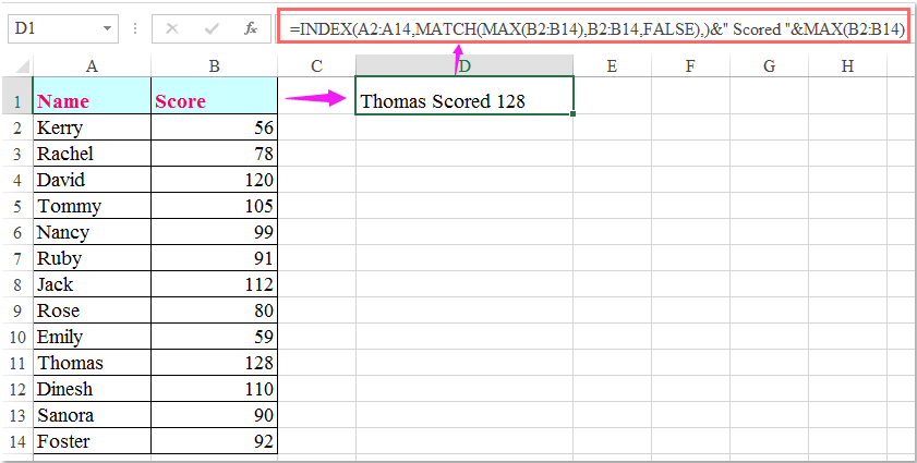
1. Inserisci la seguente formula in una cella vuota dove desideri visualizzare il nome (ad esempio, nella cella C2):
=INDEX(A2:A14,MATCH(MAX(B2:B14),B2:B14,FALSE))&" Scored "&MAX(B2:B14)Dopo aver digitato la formula, premi Invio per confermare. La formula restituirà il primo nome trovato con il punteggio più alto. Ad esempio, se sia John che Alice hanno ottenuto 98, verrà restituita solo la prima occorrenza.
Note:
1. Nella formula sopra indicata, A2:A14 è la colonna Elenco nomi da cui desideri recuperare il nome, mentre B2:B14 è l’elenco dei punteggi. Assicurati che gli intervalli corrispondano esattamente ai tuoi dati.
2. La formula restituisce solo il primo nome corrispondente. Se più persone condividono il punteggio più alto, potresti voler visualizzare tutti i nomi: consulta la soluzione pratica riportata di seguito.
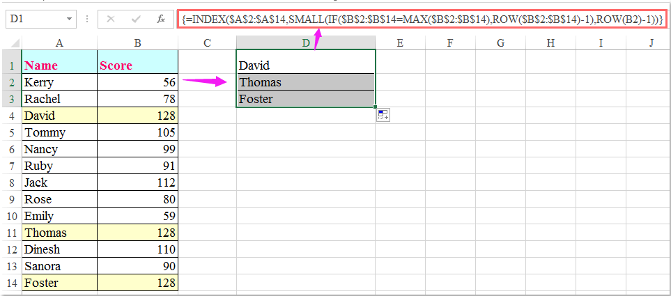
Inserisci la seguente formula in una qualsiasi cella (ad esempio D2):
=INDEX($A$2:$A$14,SMALL(IF($B$2:$B$14=MAX($B$2:$B$14),ROW($B$2:$B$14)-1),ROW(B2)-1))Dopo aver digitato la formula, premi contemporaneamente Ctrl + Maiusc + Invio (non solo Invio) per trasformarla in una formula matriciale. Apparirà il primo nome con il punteggio più alto. Seleziona quindi la cella contenente la formula e trascina il quadratino di riempimento verso il basso. Continua finché non compaiono valori di errore: ogni riga mostrerà un altro individuo con lo stesso punteggio massimo. Questo approccio è particolarmente utile in caso di parità, quando vuoi elencare tutti i vincitori.
Se la tua versione di Excel supporta le matrici dinamiche (ad esempio Office 365 o Excel 2021 e versioni successive), puoi adottare un approccio ancora più semplice. Prova a inserire questa formula in una cella e premi semplicemente Invio:
=FILTER(A2:A14,B2:B14=MAX(B2:B14))Questa formula visualizza automaticamente tutti i nomi dei migliori performer nelle celle sottostanti, senza dover trascinare o ricorrere a scorciatoie da tastiera speciali: una soluzione comoda ed efficace per le versioni più recenti di Excel.
Le formule sono potenti per ricerche rapide, ma potrebbero non essere la soluzione più adatta per set di dati molto grandi, poiché le prestazioni possono risentirne quando si gestiscono migliaia di righe. Inoltre, le formule richiedono riferimenti a intervalli coerenti per fornire risultati corretti se vengono aggiunte o rimosse righe; controlla sempre attentamente la selezione dei tuoi dati.
Codice VBA – Trova e visualizza automaticamente il/i nome/i con il punteggio più alto
L’utilizzo di macro VBA offre un metodo flessibile e automatizzato per individuare e visualizzare tutti i nomi associati al punteggio più alto nel tuo set di dati, soprattutto quando le formule risultano troppo complesse o inadeguate per elenchi estesi. Con VBA, puoi personalizzare la logica in base alle tue esigenze di reporting e gestire automaticamente gli aggiornamenti, rendendolo particolarmente efficace per analisi ripetute o elaborazioni batch.
1. Apri la tua cartella di lavoro di Excel, quindi fai clic su Sviluppo > Visual Basic. Nella finestra di Microsoft Visual Basic, Applications Edition, fai clic su Inserisci > Modulo per inserire un modulo vuoto.
Copia e incolla il seguente codice VBA nella finestra del modulo:
Sub ShowTopNames()
    Dim rngNames As Range, rngScores As Range, outCell As Range
    Dim nArr As Variant, sArr As Variant
    Dim i As Long, maxVal As Double, hasVal As Boolean
    Dim namesBuf As String
    On Error Resume Next
    Set rngNames = Application.InputBox("Please select the name column (single column)", "Top Names", Type:=8)
    Set rngScores = Application.InputBox("Please select the score column (single column, same rows as names)", "Top Names", Type:=8)
    Set outCell = Application.InputBox("Please select the output cell (optional, click Cancel to skip)", "Top Names", Type:=8)
    On Error GoTo 0
    If rngNames Is Nothing Or rngScores Is Nothing Then Exit Sub
    If rngNames.Rows.Count <> rngScores.Rows.Count Or rngNames.Columns.Count <> 1 Or rngScores.Columns.Count <> 1 Then
        MsgBox "Range mismatch: Name column and score column must be single columns with the same number of rows.", vbExclamation
        Exit Sub
    End If
    nArr = rngNames.Value2
    sArr = rngScores.Value2
    hasVal = False
    For i = 1 To UBound(sArr, 1)
        If IsNumeric(sArr(i, 1)) And Not IsEmpty(sArr(i, 1)) Then
            If Not hasVal Then
                maxVal = CDbl(sArr(i, 1))
                hasVal = True
            ElseIf CDbl(sArr(i, 1)) > maxVal Then
                maxVal = CDbl(sArr(i, 1))
            End If
        End If
    Next i
    If Not hasVal Then
        MsgBox "No valid numeric values found in the score column.", vbInformation
        Exit Sub
    End If
    rngNames.EntireRow.Interior.ColorIndex = xlNone
    For i = 1 To UBound(sArr, 1)
        If IsNumeric(sArr(i, 1)) Then
            If CDbl(sArr(i, 1)) = maxVal Then
                rngNames.Cells(i, 1).EntireRow.Interior.Color = RGB(255, 255, 153) ' Light yellow
                If Len(namesBuf) > 0 Then namesBuf = namesBuf & ", "
                namesBuf = namesBuf & CStr(nArr(i, 1))
            End If
        End If
    Next i
    If Not outCell Is Nothing Then
        outCell.Value = "Top Score: " & maxVal & " | Name(s): " & namesBuf
    End If
    MsgBox "Top Score = " & maxVal & vbCrLf & "Name(s): " & namesBuf, vbInformation, "Highest Score"
End Sub
2. Premi quindi il tasto F5 per eseguire il codice. Compariranno tre finestre di dialogo: Seleziona la colonna dei nomi (una sola colonna). Trascina per selezionare solo i nomi (ad esempio, A2:A14) → OK. Seleziona la colonna dei punteggi (una sola colonna, con lo stesso numero di righe dei nomi). Trascina per selezionare i punteggi (ad esempio, B2:B14) → OK. Seleziona la cella di output (opzionale). Fai clic su una cella di destinazione (ad esempio, D2) per inserire il risultato.
Al termine dell’esecuzione del codice, il risultato verrà visualizzato nella cella specificata e i nomi di tutti i partecipanti con il punteggio massimo saranno evidenziati in giallo chiaro nell’intera riga.
Tabella pivot – Usa una Tabella pivot per visualizzare il nome corrispondente al punteggio più alto
Le tabelle pivot in Excel offrono un modo visivo e interattivo per analizzare e riepilogare i dati. Sono particolarmente utili per gestire set di dati più ampi, eseguire analisi per gruppi e identificare rapidamente valori univoci come il massimo, ad esempio per individuare il miglior performer in ciascuna categoria o nell’intero elenco. Questo metodo non richiede formule né codifica, risultando ideale per utenti che preferiscono soluzioni basate su semplici clic del mouse e attività di reporting ricorrenti.
Il flusso di lavoro di base per utilizzare una Tabella pivot per questo scopo è il seguente:
1. Seleziona una qualsiasi cella all’interno del tuo intervallo dati (includendo sia la colonna dei nomi che quella dei punteggi), quindi vai su Inserisci > Tabella pivot. Nella finestra di dialogo, conferma l’intervallo dati e scegli se posizionare la tabella pivot in un nuovo foglio o in un foglio di lavoro esistente, in base alle tue preferenze.
2. Nel riquadro Campi tabella pivot, trascina il campo Nome nell’area Righe e il campo Punteggio nell’area Valori. Per impostazione predefinita, l’area Valori utilizzerà la funzione «Somma» o «Conteggio». Fai clic sulla freccia a discesa del campo Punteggio nell’area Valori, seleziona Impostazioni campo e scegli Max come funzione di riepilogo. Fai clic su OK.
3. Ora la Tabella pivot mostra il punteggio più alto per ciascun nome. Per evidenziare il miglior performer complessivo, ordina la colonna «Max di Punteggio» in ordine decrescente: il nome in cima sarà quello del miglior performer (o di uno dei migliori, in caso di parità). Puoi anche applicare filtri o usare la formattazione condizionale per un’enfasi visiva ancora più efficace.
Se desideri visualizzare solo i migliori performer, applica i filtri valori: fai clic sulla freccia a discesa delle etichette di riga per i nomi, seleziona Filtri valori > Uguale a e imposta il valore sul punteggio più alto (che puoi identificare ordinando temporaneamente i valori o controllando il numero più elevato nella colonna Max di Punteggio). In questo modo potrai concentrare il report esclusivamente sui nomi vincenti.
Le tabelle pivot sono strumenti potenti per l’esplorazione: puoi aggiornare, espandere o filtrare facilmente i tuoi dati, e la tabella pivot si aggiorna automaticamente per ricalcolare i risultati. Tuttavia, se il tuo set di dati cambia frequentemente, ricorda sempre di fare clic con il pulsante destro del mouse sulla tabella pivot e scegliere Aggiorna dopo aver aggiunto nuovi dati.
Le tabelle pivot richiedono una minima configurazione iniziale, ma offrono report flessibili e confronti tra gruppi — ad esempio per reparto o team — se i tuoi dati includono categorie aggiuntive.
In caso di problemi con il riepilogo o l’ordinamento, assicurati che i tuoi dati non contengano celle vuote e che i nomi delle condizioni siano scritti in modo coerente. Quando utilizzi elenchi estesi, presta attenzione all’intervallo di origine: questo garantisce che la tabella pivot includa tutti i dati correlati.

Sblocca la magia di Excel con KUTOOLS AI
- Esecuzione intelligente: Esegui operazioni sulle celle, analizza i dati e crea grafici, il tutto con comandi semplici e intuitivi.
- Formule personalizzate: crea formule su misura per ottimizzare i tuoi flussi di lavoro.
- Codifica VBA: Scrivi e implementa codice VBA in modo semplice e immediato.
- Interpretazione delle formule: Comprendi con facilità anche le formule più complesse.
- Traduzione del testo: Superate le barriere linguistiche direttamente nei vostri fogli di calcolo.
Migliori Strumenti per la Produttività in Office
Potenzia le tue competenze in Excel con Kutools per Excel e sperimenta un’efficienza mai vista prima.Kutools per Excel offre oltre 300 funzionalità avanzate per aumentare la produttività e Risparmia tempo.Clicca qui per ottenere la funzionalità di cui hai più bisogno...
Office Tab Porta l'interfaccia a schede in Office e rende il tuo lavoro molto più semplice
- Abilita la modifica e la lettura a schede in Word, Excel, PowerPoint, Publisher, Access, Visio e Project.
- Apri e crea più documenti in nuove schede all’interno della stessa finestra, invece che in finestre separate.
- Aumenta la tua produttività del 50 % e risparmia centinaia di clic del mouse ogni giorno!
Tutti i componenti aggiuntivi di Kutools in un unico programma di installazione.
Kutools for Office è la suite che include componenti aggiuntivi per Excel, Word, Outlook e PowerPoint, oltre a Office Tab Pro: la soluzione ideale per i team che lavorano su diverse app di Office.
- Suite completa— componenti aggiuntivi per Excel, Word, Outlook e PowerPoint + Office Tab Pro
- Un unico programma di installazione, una sola licenza— configurazione in pochi minuti (pronto per MSI)
- Funziona meglio insieme— produttività ottimizzata tra le app di Office
- Prova gratuita di 30 giorni con tutte le funzionalità— nessuna registrazione, nessuna carta di credito
- Miglior rapporto qualità-prezzo— risparmia rispetto all’acquisto dei singoli componenti aggiuntivi