Come trovare la n-esima cella non vuota in Excel?
Come trovare e restituire il valore della n-esima cella non vuota in una colonna o riga di Excel? In questo articolo ti mostrerò alcune formule efficaci per portare a termine questo compito con facilità.
Trova e restituisci il valore della n-esima cella non vuota da una colonna con una formula
Trova e restituisci il valore della n-esima cella non vuota da una riga con una formula
 Trova e restituisci il valore della n-esima cella non vuota da una colonna con una formula
Ad esempio, ho una colonna di dati come mostrato nello screenshot seguente e ora voglio recuperare il valore della terza cella non vuota di questo elenco.
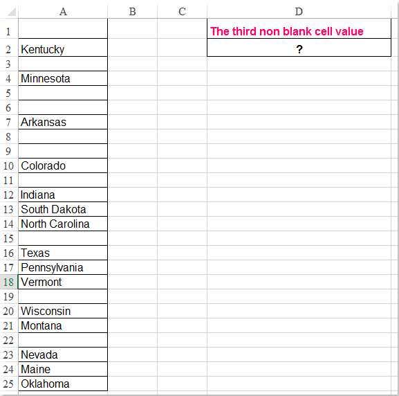
Inserisci questa formula:=INDEX($A$1:$A$25,SMALL(ROW($A$1:$A$25)+(100*($A$1:$A$25=«»)), 3))&""in una cella vuota in cui desideri visualizzare il risultato, ad esempio D2, quindi premi contemporaneamente i tasti Ctrl + Maiusc + Invioper ottenere il risultato corretto, vedi screenshot:

Nota: Nella formula precedente, A1:A25 è l'elenco di dati che desideri utilizzare e il numero 3 indica il valore della terza cella non vuota che vuoi restituire. Se desideri ottenere la seconda cella non vuota, modifica semplicemente il numero 3 in 2, adattandolo alle tue esigenze.
Trova e restituisci il valore della n-esima cella non vuota da una riga con una formula
Se desideri trovare e restituire il valore della n-esima cella non vuota in una riga, la formula seguente potrebbe esserti utile; procedi nel modo seguente:
Inserisci questa formula:=INDEX($A$1:$M$1,SMALL(IF($A$1:$M$1<>«»,COLUMN($A$1:$M$1)-COLUMN($A$1)+1),4))in una cella vuota in cui desideri visualizzare il risultato, quindi premi contemporaneamente i tasti Ctrl + Maiusc + Invioper ottenere il risultato, vedi screenshot:
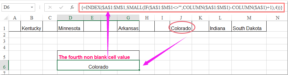
Nota: Nella formula precedente, A1:M1 sono i valori della riga che desideri utilizzare e il numero 4 indica il valore della quarta cella non vuota che vuoi restituire. Se desideri ottenere la seconda cella non vuota, modifica semplicemente il numero 4 in 2, secondo necessità.
Migliori Strumenti per la Produttività in Office
Potenzia le tue competenze in Excel con Kutools per Excel e sperimenta un’efficienza mai vista prima.Kutools per Excel offre oltre 300 funzionalità avanzate per aumentare la produttività e Risparmia tempo.Clicca qui per ottenere la funzionalità di cui hai più bisogno...
Office Tab Porta l'interfaccia a schede in Office e rende il tuo lavoro molto più semplice
- Abilita la modifica e la lettura a schede in Word, Excel, PowerPoint, Publisher, Access, Visio e Project.
- Apri e crea più documenti in nuove schede all’interno della stessa finestra, invece che in finestre separate.
- Aumenta la tua produttività del 50 % e risparmia centinaia di clic del mouse ogni giorno!
Tutti i componenti aggiuntivi di Kutools in un unico programma di installazione.
Kutools for Office è la suite che include componenti aggiuntivi per Excel, Word, Outlook e PowerPoint, oltre a Office Tab Pro: la soluzione ideale per i team che lavorano su diverse app di Office.
- Suite completa— componenti aggiuntivi per Excel, Word, Outlook e PowerPoint + Office Tab Pro
- Un unico programma di installazione, una sola licenza— configurazione in pochi minuti (pronto per MSI)
- Funziona meglio insieme— produttività ottimizzata tra le app di Office
- Prova gratuita di 30 giorni con tutte le funzionalità— nessuna registrazione, nessuna carta di credito
- Miglior rapporto qualità-prezzo— risparmia rispetto all’acquisto dei singoli componenti aggiuntivi