Vai al contenuto principale

Come sommare in base ai criteri di colonna e riga in Excel? 

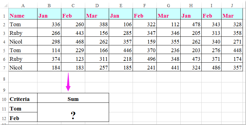
Ho un intervallo di dati che contiene intestazioni di riga e di colonna, ora voglio prendere una somma delle celle che soddisfano i criteri di intestazione di colonna e riga. Ad esempio, per sommare le celle il cui criterio di colonna è Tom e il criterio di riga è Feb come mostrato nella seguente schermata. In questo articolo parlerò di alcune formule utili per risolverlo.

doc sum colonna riga criteri 1

Somma le celle in base ai criteri di colonna e riga con le formule


freccia blu freccia destra Somma le celle in base ai criteri di colonna e riga con le formule

Qui puoi applicare le seguenti formule per sommare le celle in base ai criteri di colonna e riga, per favore fai come segue:

Immettere una delle seguenti formule in una cella vuota in cui si desidera visualizzare il risultato:

=SUMPRODUCT((A2:A7="Tom")*(B1:J1="Feb")*(B2:J7))

=SUM(IF(B1:J1="Feb",IF(A2:A7="Tom",B2:J7)))

E poi premere Maiusc + Ctrl + Invio tasti insieme per ottenere il risultato, vedi screenshot:
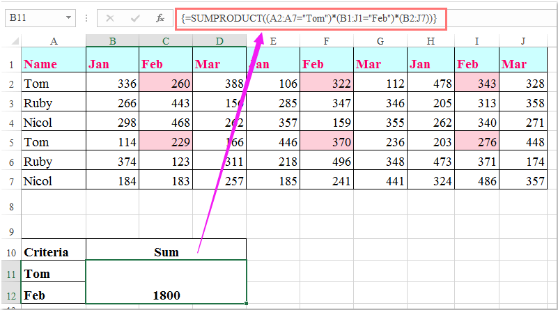
doc sum colonna riga criteri 2

Note:: Nelle formule precedenti: Tom ed Febbraio sono i criteri di colonna e di riga basati su, A2: A7, B1: J1 sono le intestazioni di colonna e le intestazioni di riga contengono i criteri, B2: J7 è l'intervallo di dati che desideri sommare.

I migliori strumenti per la produttività in ufficio

🤖 Assistente AI di Kutools: Rivoluziona l'analisi dei dati basandosi su: Esecuzione intelligente   |  Genera codice  |  Crea formule personalizzate  |  Analizzare i dati e generare grafici  |  Richiama le funzioni di Kutools...
Funzioni popolari: Trova, evidenzia o identifica i duplicati   |  Elimina righe vuote   |  Combina colonne o celle senza perdere dati   |   Round senza formula ...
Super ricerca: VLookup a criteri multipli    VLookup a valori multipli  |   VLookup su più fogli   |   Ricerca fuzzy ....
Elenco a discesa avanzato: Crea rapidamente un elenco a discesa   |  Elenco a discesa dipendente   |  Elenco a discesa a selezione multipla ....
Gestore di colonna: Aggiungi un numero specifico di colonne  |  Sposta colonne  |  Attiva/disattiva lo stato di visibilità delle colonne nascoste  |  Confronta intervalli e colonne ...
Funzionalità in primo piano: Messa a fuoco della griglia   |  Vista di progettazione   |   Grande barra delle formule    Gestore di cartelle di lavoro e fogli   |  Resource Library (Testo automatico)   |  Date picker   |  Combina fogli di lavoro   |  Crittografa/decrittografa le celle    Invia e-mail per elenco   |  Super filtro   |   Filtro speciale (filtro grassetto/corsivo/barrato...) ...
I 15 migliori set di strumenti12 Testo Strumenti (aggiungi testo, Rimuovi personaggi, ...)   |   50+ Grafico Tipi (Diagramma di Gantt, ...)   |   40+ Pratico Formule (Calcola l'età in base al compleanno, ...)   |   19 Inserimento Strumenti (Inserisci il codice QR, Inserisci immagine dal percorso, ...)   |   12 Conversione Strumenti (Numeri in parole, Conversione di valuta, ...)   |   7 Unisci e dividi Strumenti (Combina righe avanzate, Celle divise, ...)   |   ... e altro ancora

Potenzia le tue competenze di Excel con Kutools per Excel e sperimenta l'efficienza come mai prima d'ora. Kutools per Excel offre oltre 300 funzionalità avanzate per aumentare la produttività e risparmiare tempo.  Fai clic qui per ottenere la funzionalità di cui hai più bisogno...

Descrizione


Office Tab porta l'interfaccia a schede in Office e semplifica notevolmente il tuo lavoro

  • Abilita la modifica e la lettura a schede in Word, Excel, PowerPoint, Publisher, Access, Visio e Project.
  • Apri e crea più documenti in nuove schede della stessa finestra, piuttosto che in nuove finestre.
  • Aumenta la produttività del 50% e riduce ogni giorno centinaia di clic del mouse!
Comments (17)
No ratings yet. Be the first to rate!
This comment was minimized by the moderator on the site
Brilliant!

The function =SUM(IF(B1:J1="Feb",IF(A2:A7="Tom",B2:J7))) is a great X & Y summation tool.
I would not have thought this logic out on my own.
In fact i took me a minute to deconstruction the operations.

Thank you
This comment was minimized by the moderator on the site
My data that I am trying to retrieve is in a table. Would this impact the result at all? I have:

=SUM(IF('[Primary Controller Active Project Database (KC notes)1.xlsx]Active Project Tracking'!$B2:$B66=X2,IF('[Primary Controller Active Project Database (KC notes)1.xlsx]Active Project Tracking'!$A1:$AV1=AH10,'[Primary Controller Active Project Database (KC notes)1.xlsx]Active Project Tracking'!$H$2:$AV$66)))

So I think the equivalent would be if you did your information above, but in a table in a different workbook. Thoughts?
This comment was minimized by the moderator on the site
If there were negatives in the matrix and you only wanted to include the positives, what would you do? 
I tried to do something like this:

=SUMPRODUCT((Column = Criteria)* ( Row = Criteria) * (second column = Criteria) * (Matrix) * (Matrix >0))

This comment was minimized by the moderator on the site
Is there a way to do this but instead of writing "Tom" & "Feb" in the formula, you are able to reference the criteria cells e.g.A11 & A12?
This comment was minimized by the moderator on the site
Hello, Rianna,Yest, as you said, you can use the cell references to replace the text in the formula, such as:
=SUMPRODUCT((A2:A7=A2)*(B1:J1=C1)*(B2:J7))
=SUM(IF(B1:J1=C1,IF(A2:A7=A2,B2:J7)))
This comment was minimized by the moderator on the site
In the above example which formula should I use if I wanted calculate the sum of the amounts earned by Tom Ruby & Nicol in March?
This comment was minimized by the moderator on the site
Hello, Nabar,To get the result you want, please apply the below formula:=SUMPRODUCT(((A2:A7="Tom")+(A2:A7="Nicol")+(A2:A7="Ruby"))*(B1:J1="Mar")*(B2:J7))
Please try, hope it can help you!
This comment was minimized by the moderator on the site
Hello Skyyang,
Thank you for your response. I tried the formula you suggested but I am not getting the right answer. Probably I wasn't able to put my query correctly. Let me try again I have a spreadsheet with data with daily calculation, I have numbered the first row 1,2,3,4.....132. 2nd, 3rd 4th &5th rows has table headings. The first column has line no's numbered 1, 2,3,.....3005 starting from row 6,range B6:EF3005 has data filled in on everyday basis. In second sheet i have a table in which I want to apply a formula which will look up two line numbers fed in two different rows and calculate the sum from the range B6: EF3005 from the data spreadsheet between the two line numbers from a certain column viz sum of values in column 15 between rows (line No's) 50 & 85.
This comment was minimized by the moderator on the site
Is there a way to make this work with wildcard characters? I'd like to use it on everything starting with certain characters, but with (a fixed number of) undefined characters at the end, i.e. =SUM(IF(B1:J1="Fe*",IF(A2:A7="To*",B2:J7)))
This comment was minimized by the moderator on the site
Should anyone have the same question, this is how I solved it (in Google Sheets, not tested in Excel):

=ArrayFormula(SUM(IF(regexmatch(O5:W5,"^Fe."),IF(regexmatch(N6:N11,"^To."),O6:W11))))

Note that the IF function does not support wildcard characters and that for regexmatch the wildcards are different and can be found here: https://github.com/google/re2/blob/master/doc/syntax.txt
In this particular instance, I used ^ to indicate that Fe & Tom occur at the beginning of text and . to allow for any following character (* would mean zero or more of the previous character, e.g. Fe* would only look for instances with 1 or more "e"s after F)
This comment was minimized by the moderator on the site
I tried to create a formula to calculate if the D12 is blank, it will calculate from K12 to AH12 but it seems this part ' regexmatch(D12,"")' is not working
ArrayFormula(SUM(IF(regexmatch(D12,""),K12:AH12)))
This comment was minimized by the moderator on the site
Thank you so much! You made my day!! @TeSageDS
This comment was minimized by the moderator on the site
how would you do this same formula if you wanted to sum both Feb and March together? please help! thanks

=SUMPRODUCT((A2:A7="Tom")*(B1:J1="Feb")*(B2:J7))
This comment was minimized by the moderator on the site
Hello,Angela,
To solve your problem, you just need to apply the below formula, please try it.

=SUMPRODUCT((A2:A7="Tom")*((B1:J1="Feb")+(B1:J1="Mar"))*(B2:J7)).

Hope it can help you!
This comment was minimized by the moderator on the site
Brilliant
This comment was minimized by the moderator on the site
Worth pointing out that of the two formulas provided above you do not need to enter the SUMPRODUCT formula with Ctrl + Shift + Enter. It will work perfectly well without it.
This comment was minimized by the moderator on the site
Awesome, this is the one what i was looking for. thanks for the help
There are no comments posted here yet
Please leave your comments in English
Posting as Guest
×
Rate this post:
0   Characters
Suggested Locations