Come creare un elenco a discesa dipendente in Google Fogli?
Inserire un normale elenco a discesa in Google Sheets potrebbe sembrarti semplice, ma a volte ti servirà creare un elenco dinamico, in cui le opzioni del secondo elenco cambiano in base alla selezione effettuata nel primo. Come puoi realizzare questa funzionalità in Google Sheets?
Crea un elenco a discesa dipendente in Google Sheets
Crea un elenco a discesa dipendente in Google Sheets
Segui questi passaggi per creare un Elenco dinamico in Google Sheets:
1. Innanzitutto, inserisci l’elenco a discesa di base: seleziona una cella in cui desideri posizionare il primo elenco a discesa, quindi fai clic su Dati > Convalida dati. Vedi screenshot:

2. Nella finestra di dialogo Convalida dati visualizzata, seleziona Elenco da un intervallo dall’elenco a discesa accanto alla sezione Criteri, quindi fai clic sul pulsante per selezionare le celle contenenti i valori su cui basare il primo elenco a discesa. Vedi screenshot: 

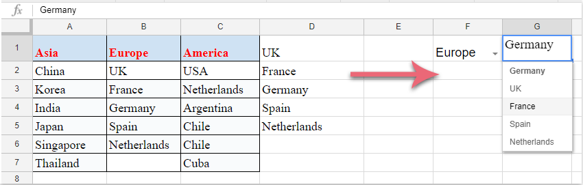
3. Clicca quindi su Salva e il primo elenco a discesa sarà creato. Scegli un elemento dall’elenco appena creato, quindi inserisci questa formula: =arrayformula(if(F1=A1,A2:A7,if(F1=B1,B2:B6,if(F1=C1,C2:C7,«»)))) in una cella vuota adiacente alle colonne dei dati, poi premi il tasto Invio: tutti i valori corrispondenti all’elemento selezionato nel primo elenco a discesa verranno visualizzati immediatamente. Vedi screenshot:
Nota: Nella formula indicata sopra, F1 è la cella del primo elenco a discesa; A1, B1 e C1 sono gli elementi del primo elenco a discesa; A2:A7, B2:B6 e C2:C7 sono i valori delle celle su cui si basa il secondo elenco a discesa. Puoi modificarli in base alle tue esigenze.

4. A questo punto puoi creare il secondo elenco a discesa dipendente: fai clic su una cella in cui desideri inserire il secondo elenco a discesa, quindi clicca su Dati > Convalida dati per aprire la finestra di dialogo Convalida dati. Scegli Elenco da un intervallo dall’elenco a discesa accanto alla sezione Criteri, quindi fai clic sul pulsante per selezionare le celle contenenti la formula con i risultati corrispondenti all’elemento scelto nel primo elenco. Vedi screenshot:

5. Infine, fai clic sul pulsante Salva e il secondo elenco a discesa dipendente verrà creato correttamente, come mostrato nello screenshot seguente:
Migliori Strumenti per la Produttività in Office
Potenzia le tue competenze in Excel con Kutools per Excel e sperimenta un’efficienza mai vista prima.Kutools per Excel offre oltre 300 funzionalità avanzate per aumentare la produttività e Risparmia tempo.Clicca qui per ottenere la funzionalità di cui hai più bisogno...
Office Tab Porta l'interfaccia a schede in Office e rende il tuo lavoro molto più semplice
- Abilita la modifica e la lettura a schede in Word, Excel, PowerPoint, Publisher, Access, Visio e Project.
- Apri e crea più documenti in nuove schede all’interno della stessa finestra, invece che in finestre separate.
- Aumenta la tua produttività del 50 % e risparmia centinaia di clic del mouse ogni giorno!
Tutti i componenti aggiuntivi di Kutools in un unico programma di installazione.
Kutools for Office è la suite che include componenti aggiuntivi per Excel, Word, Outlook e PowerPoint, oltre a Office Tab Pro: la soluzione ideale per i team che lavorano su diverse app di Office.
- Suite completa— componenti aggiuntivi per Excel, Word, Outlook e PowerPoint + Office Tab Pro
- Un unico programma di installazione, una sola licenza— configurazione in pochi minuti (pronto per MSI)
- Funziona meglio insieme— produttività ottimizzata tra le app di Office
- Prova gratuita di 30 giorni con tutte le funzionalità— nessuna registrazione, nessuna carta di credito
- Miglior rapporto qualità-prezzo— risparmia rispetto all’acquisto dei singoli componenti aggiuntivi