Come usare CERCA.VERT per restituire sia il valore cercato che il relativo colore di sfondo in Excel?
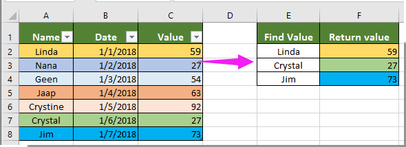
Supponiamo che tu abbia una tabella come quella mostrata nell’immagine seguente. Ora vuoi verificare se un determinato valore è presente nella colonna A e, in tal caso, restituire il valore corrispondente insieme al suo colore di sfondo nella colonna C. Come fare? Il metodo descritto nell’articolo ti aiuterà a risolvere questo problema.
CERCA.VERT e restituzione di Colore di Sfondo con il valore cercato mediante funzione definita dall’utente
Procedi come segue per cercare un valore e restituire il valore corrispondente insieme al suo Colore di Sfondo in Excel.
1. Nel foglio di lavoro che contiene il valore da cercare con CERCA.VERT, fai clic con il pulsante destro del mouse sulla scheda del foglio e seleziona Visualizza codice dal menu contestuale. Vedi immagine:

2. Nella finestra di Microsoft Visual Basic, Applications Edition aperta, copia il seguente codice VBA nella finestra del codice.
Codice VBA 1: CERCA.VERT e restituzione di Colore di Sfondo con il valore cercato
Sub Worksheet_Change(ByVal Target As Range)
    Dim I As Long
    Dim xKeys As Long
    Dim xDicStr As String
    On Error Resume Next
    Application.ScreenUpdating = False
    xKeys = UBound(xDic.Keys)
    If xKeys >= 0 Then
        For I = 0 To UBound(xDic.Keys)
            xDicStr = xDic.Items(I)
            If xDicStr <> "" Then
                Range(xDic.Keys(I)).Interior.Color = _
                Range(xDic.Items(I)).Interior.Color
            Else
                Range(xDic.Keys(I)).Interior.Color = xlNone
            End If
        Next
        Set xDic = Nothing
    End If
    Application.ScreenUpdating = True
End Sub
3. Quindi fai clic su Inserisci > Modulo e copia il seguente codice VBA 2 nella finestra del modulo.
Codice VBA 2: CERCA.VERT e restituzione di Colore di Sfondo con il valore cercato
Public xDic As New Dictionary
Function LookupKeepColor (ByRef FndValue, ByRef LookupRng As Range, ByRef xCol As Long)
    Dim xFindCell As Range
    On Error Resume Next
    Set xFindCell = LookupRng.Find(FndValue, , xlValues, xlWhole)
    If xFindCell Is Nothing Then
        LookupKeepColor = ""
        xDic.Add Application.Caller.Address, ""
    Else
        LookupKeepColor = xFindCell.Offset(0, xCol - 1).Value
        xDic.Add Application.Caller.Address, xFindCell.Offset(0, xCol - 1).Address
    End If
End Function
4. Dopo aver inserito i due codici, fai clic su Strumenti > Riferimenti. Quindi, seleziona la casella Microsoft Script Runtime nella finestra di dialogo Riferimenti – VBAProject. Vedi immagine:

5. Premi i tasti Alt+Q per chiudere la finestra di Microsoft Visual Basic, Applications Edition e tornare al foglio di lavoro.
6. Seleziona una cella vuota accanto al valore da cercare, quindi inserisci la formula =LookupKeepColor(E2;$A$1:$C$8;3) nella Barra delle formule e premi Invio.

Nota: Nella formula, E2 contiene il valore da cercare, $A$1:$C$8 è l’intervallo della tabella e il numero 3 indica che il valore corrispondente da restituire si trova nella terza colonna della tabella. Modificali in base alle tue esigenze.
7. Mantieni selezionata la prima cella del risultato e trascina il quadratino di riempimento verso il basso per ottenere tutti i risultati con il relativo colore di sfondo. Vedi immagine.

Articoli correlati:
- Come si fa a copiare la formattazione della cella di origine quando si utilizza CERCA.VERT in Excel?
- Come usare CERCA.VERT in Excel per restituire un valore formattato come data invece che come numero?
- Come si utilizzano insieme CERCA.VERT e SOMMA in Excel?
- Come usare CERCA.VERT per restituire un valore dalla cella adiacente o successiva in Excel?
- Come cercare un valore con CERCA.VERT e restituire VERO o FALSO (o SÌ o NO) in Excel?
Migliori Strumenti per la Produttività in Office
Potenzia le tue competenze in Excel con Kutools per Excel e sperimenta un’efficienza mai vista prima.Kutools per Excel offre oltre 300 funzionalità avanzate per aumentare la produttività e Risparmia tempo.Clicca qui per ottenere la funzionalità di cui hai più bisogno...
Office Tab Porta l'interfaccia a schede in Office e rende il tuo lavoro molto più semplice
- Abilita la modifica e la lettura a schede in Word, Excel, PowerPoint, Publisher, Access, Visio e Project.
- Apri e crea più documenti in nuove schede all’interno della stessa finestra, invece che in finestre separate.
- Aumenta la tua produttività del 50 % e risparmia centinaia di clic del mouse ogni giorno!
Tutti i componenti aggiuntivi di Kutools in un unico programma di installazione.
Kutools for Office è la suite che include componenti aggiuntivi per Excel, Word, Outlook e PowerPoint, oltre a Office Tab Pro: la soluzione ideale per i team che lavorano su diverse app di Office.
- Suite completa— componenti aggiuntivi per Excel, Word, Outlook e PowerPoint + Office Tab Pro
- Un unico programma di installazione, una sola licenza— configurazione in pochi minuti (pronto per MSI)
- Funziona meglio insieme— produttività ottimizzata tra le app di Office
- Prova gratuita di 30 giorni con tutte le funzionalità— nessuna registrazione, nessuna carta di credito
- Miglior rapporto qualità-prezzo— risparmia rispetto all’acquisto dei singoli componenti aggiuntivi