Restituisci più valori corrispondenti in base a più criteri in Excel (Guida completa)
Gli utenti di Excel si trovano spesso di fronte a scenari in cui devono estrarre più valori che soddisfano contemporaneamente diversi criteri, presentando tutti i risultati in una colonna, una riga o in un’unica cella consolidata. Questa guida illustra metodi compatibili con tutte le versioni di Excel, oltre alla nuova funzione FILTRO disponibile in Excel 365 e 2021.
Restituisci più valori corrispondenti in base a più criteri in un’unica cella
In Excel, estrarre più valori corrispondenti in base a più criteri all’interno di un’unica cella è una sfida comune. Di seguito sono illustrate due metodologie efficienti.
Metodo 1: Utilizzo della funzione TESTO.UNISCI (Excel 365 / 2021,2019)
Per ottenere tutti i valori corrispondenti in un’unica cella separati da delimitatori, la funzione TESTO.UNISCI può rivelarsi davvero preziosa.
Inserisci o copia la seguente formula in una cella vuota, quindi premi Invio (Excel 2021 e Excel 365) oppure Ctrl + Maiusc + Invio in Excel 2019 per ottenere il risultato:
=TEXTJOIN(", ", TRUE, IF(($A$2:$A$18=E2)*($B$2:$B$18=F2), $C$2:$C$18, ""))
- ($A$2:$A$21=E2)*($B$2:$B$21=F2) verifica se ogni riga soddisfa entrambe le condizioni: «venditore uguale a E2» e «mese uguale a F2». Quando entrambe le condizioni sono vere, il risultato è 1; altrimenti, è 0. L’asterisco * indica che devono essere soddisfatte contemporaneamente.
- SE(..., $C$2:$C$21, «») restituisce il nome del prodotto se la riga corrisponde; altrimenti, restituisce una cella vuota.
- TESTO.UNISCI(", ", VERO, ...) unisce tutti i nomi di prodotto non vuoti in un’unica cella, separati da ", ".
Metodo 2: Utilizzo di Kutools per Excel
Kutools per Excel offre una soluzione potente e semplice, che ti permette di recuperare e combinare rapidamente più corrispondenze in un’unica cella in base a diversi criteri, senza dover ricorrere a formule complesse.
Dopo aver installato Kutools per Excel, procedi come segue:
- Seleziona l’intervallo di dati da cui desideri ottenere tutti i valori corrispondenti in base ai criteri.
- Quindi, fai clic su Kutools > Unisci e Dividi > Unione avanzata righe, vedi screenshot:

- Nella finestra di dialogo Unione avanzata righe, configura le seguenti opzioni:
- Seleziona le intestazioni di colonna che contengono i tuoi criteri di ricerca (ad esempio, Venditore e Mese). Per ogni colonna selezionata, clicca su Chiave primaria per impostarla come condizione di ricerca.
- Fai clic sull’intestazione della colonna in cui desideri ottenere i Risultati uniti (ad esempio, Prodotto). Nella sezione Combina, seleziona il delimitatore preferito, come virgola, spazio o un separatore personalizzato.
- Infine, clicca sul pulsante OK.


Risultato: Kutools unirà immediatamente tutti i valori corrispondenti in un’unica cella per ogni combinazione univoca dei criteri.
Restituisci più valori corrispondenti in base a più criteri in una colonna
Quando devi estrarre e visualizzare più record corrispondenti da un set di dati in base a diverse condizioni, con risultati presentati in formato verticale, Excel ti offre diverse soluzioni efficaci.
Metodo 1: Utilizzo di una formula matriciale (per tutte le versioni)
Puoi utilizzare la seguente formula matriciale per restituire i risultati in verticale in una colonna:
1. Copia o inserisci la seguente formula in una cella vuota:
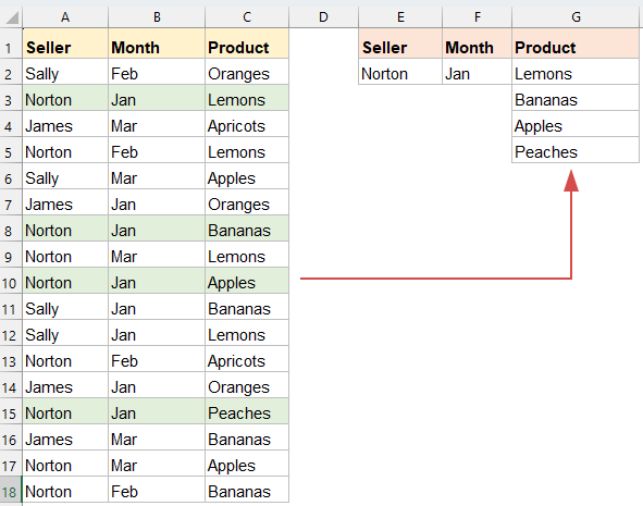
=IFERROR(INDEX($C$2:$C$18, SMALL(IF(($A$2:$A$18=$E$2)*($B$2:$B$18=$F$2), ROW($C$2:$C$18)-ROW($C$2)+1), ROW(1:1))), "")2. Premi Ctrl + Maiusc + Invio per ottenere il primo risultato corrispondente, quindi seleziona la prima cella contenente la formula e trascina il quadratino di riempimento verso il basso finché non appare una cella vuota. A quel punto, tutti i valori corrispondenti saranno visualizzati, come mostrato nello screenshot seguente:

- $A$2:$A$18=$E$2: Verifica se il venditore corrisponde al valore nella cella E2.
- $B$2:$B$18=$F$2: Verifica se il mese corrisponde al valore nella cella F2.
- * è un operatore logico AND (entrambe le condizioni devono essere vere).
- RIGA($C$2:$C$18)-RIGA($C$2)+1: genera un numero di riga relativo per ogni prodotto.
- PICCOLO(..., RIGA(1:1)): Recupera l’n-esima riga corrispondente più piccola (man mano che la formula viene trascinata verso il basso).
- INDICE(...): Restituisce il valore corrispondente dalla riga indicata.
- SE.ERRORE(..., «»): Restituisce una cella vuota quando non ci sono altre corrispondenze.
Metodo 2: Utilizzo della funzione FILTRO (Excel 365 / 2021)
Se utilizzi Excel 365 o Excel 2021, la funzione FILTRO è la scelta ideale per ottenere risultati multipli in base a criteri multipli: semplice, chiara e capace di espandere dinamicamente i risultati senza ricorrere a formule matriciali complesse.
Copiare o incollare la seguente formula in una cella vuota, quindi premere Invio: tutti i record corrispondenti verranno restituiti in base ai criteri multipli.
=FILTER(C2:C18, (A2:A18=E2)*(B2:B18=F2), "No match")
- FILTRO(...) restituisce tutti i valori da C2:C18 per cui entrambe le condizioni sono soddisfatte.
- (A2:A18=E2)*(B2:B18=F2): matrice logica che verifica la corrispondenza tra venditore e mese.
- «Nessuna corrispondenza»: messaggio opzionale visualizzato quando non vengono trovati valori.
Restituisci più valori corrispondenti in base a più criteri in una riga
Gli utenti di Excel spesso devono estrarre più valori da un set di dati che soddisfano diverse condizioni e disporli orizzontalmente (in una riga). Questo approccio è ideale per creare report dinamici, dashboard o tabelle riepilogative quando lo spazio verticale è limitato. In questa sezione esploreremo due metodi efficaci.
Metodo 1: Utilizzo di una formula matriciale (per tutte le versioni)
Le tradizionali formule matriciali permettono di estrarre più valori corrispondenti combinando le funzioni INDICE, PICCOLO, SE e COLONNA. A differenza dell’estrazione verticale (basata sulle colonne), adattiamo la formula per restituire i risultati su una riga.
1. Copia o inserisci la seguente formula in una cella vuota:
=IFERROR(INDEX($C$2:$C$18, SMALL(IF(($A$2:$A$18=$E$2)*($B$2:$B$18=$F$2), ROW($C$2:$C$18)-ROW($C$2)+1), COLUMN(A1))), "")2. Premere Ctrl + Maiusc + Invio per ottenere il primo risultato corrispondente, quindi selezionare la prima cella contenente la formula e trascinarla verso destra attraverso le colonne per recuperare tutti i risultati.

- $A$2:$A$18=$E$2: Verifica se il venditore corrisponde.
- $B$2:$B$18=$F$2: Verifica se il mese corrisponde.
- *: Operatore logico AND — entrambe le condizioni devono essere vere.
- RIGA($C$2:$C$18)-RIGA($C$2)+1: Genera numeri di riga relativi e imposta il conteggio delle righe.
- COLONNA(A1): Determina quale corrispondenza restituire in base a quanto la formula è stata trascinata verso destra.
- SE.ERRORE(...): Evita errori quando le corrispondenze si esauriscono.
Metodo 2: Utilizzo della funzione FILTRO (Excel 365 / 2021)
Copiare o incollare la seguente formula in una cella vuota, quindi premere Invio: tutti i valori corrispondenti verranno estratti e disposti su un’unica riga. Vedere lo screenshot:
=TRANSPOSE(FILTER(C2:C18, (A2:A18=E2)*(B2:B18=F2), "No match"))
- FILTRO(...): Recupera i valori corrispondenti dalla colonna C in base a due condizioni.
- (A2:A18=E2)*(B2:B18=F2): Entrambe le condizioni devono essere vere.
- TRASPOSTA(...): Trasforma la matrice verticale restituita da FILTRO in una matrice orizzontale.
🔚 Conclusione
Il recupero di più valori corrispondenti in base a criteri multipli in Excel può essere effettuato in diversi modi, a seconda di come si preferisce visualizzare i risultati: in una colonna, in una riga o all’interno di una singola cella.
- Per gli utenti di Excel 365 o Excel 2021, la funzione FILTRO offre una soluzione moderna, dinamica ed elegante che riduce al minimo la complessità.
- Per chi utilizza versioni precedenti, le formule matriciali restano strumenti potenti, pur richiedendo un’impostazione e un’attenzione leggermente superiori.
- Inoltre, se desideri consolidare i risultati in un’unica cella o preferisci una soluzione senza codice, la funzione TESTO.UNISCI o strumenti di terze parti come Kutools per Excel possono semplificare notevolmente il processo.
Scegliere il metodo più adatto alla propria versione di Excel e al layout preferito ti permette di gestire ricerche con criteri multipli in modo efficiente e preciso. Se vuoi scoprire altri suggerimenti e trucchi per Excel, il nostro sito web offre migliaia di tutorial per padroneggiare Excel.
Altri articoli correlati:
- Restituisci più Intervallo di valore di ricerca in un’unica cella separati da virgole
- In Excel, possiamo usare la funzione CERCA.VERT per restituire il primo valore corrispondente da una tabella, ma a volte dobbiamo estrarre tutti i valori corrispondenti e unirli in un’unica cella, separati da un delimitatore specifico come una virgola, un trattino o altro, come illustrato nello screenshot seguente. Come possiamo recuperare e restituire tutti i valori corrispondenti all’intervallo di ricerca in un’unica cella, separati da virgole, in Excel?
- Cerca.vert e restituisci più valori corrispondenti contemporaneamente nel foglio Google
- La normale funzione CERCA.VERT in Google Fogli ti permette di trovare e restituire solo il primo valore corrispondente in base a un dato fornito. Tuttavia, a volte potresti aver bisogno di cercare e restituire *tutti* i valori corrispondenti, come mostrato nello screenshot seguente. Conosci metodi semplici ed efficaci per risolvere questo compito in Google Fogli?
- Cerca.vert e restituisci più valori da un elenco a discesa
- In Excel, come puoi cercare e restituire più valori corrispondenti da un elenco a discesa, in modo da visualizzare immediatamente tutti i valori associati non appena selezioni un elemento dall’elenco, come illustrato nello screenshot seguente? In questo articolo ti guiderò passo dopo passo verso la soluzione.
- Cerca.vert e restituisci più valori in verticale in Excel
- Di solito, puoi usare la funzione CERCA.VERT per ottenere il primo valore corrispondente, ma a volte potresti aver bisogno di restituire tutti i record che soddisfano un criterio specifico. In questo articolo ti spiegherò come cercare e recuperare tutti i valori corrispondenti in verticale, in orizzontale o all’interno di un’unica cella.
- Cerca.vert e restituisci dati corrispondenti compresi tra due valori in Excel
- In Excel, possiamo utilizzare la normale funzione CERCA.VERT per recuperare il valore corrispondente in base a un dato specifico. Tuttavia, capita spesso di dover cercare e restituire un valore compreso tra due numeri, come illustrato nello screenshot seguente. Come puoi affrontare questa situazione in Excel?
Migliori Strumenti per la Produttività in Office
Potenzia le tue competenze in Excel con Kutools per Excel e sperimenta un’efficienza mai vista prima.Kutools per Excel offre oltre 300 funzionalità avanzate per aumentare la produttività e Risparmia tempo.Clicca qui per ottenere la funzionalità di cui hai più bisogno...
Office Tab Porta l'interfaccia a schede in Office e rende il tuo lavoro molto più semplice
- Abilita la modifica e la lettura a schede in Word, Excel, PowerPoint, Publisher, Access, Visio e Project.
- Apri e crea più documenti in nuove schede all’interno della stessa finestra, invece che in finestre separate.
- Aumenta la tua produttività del 50 % e risparmia centinaia di clic del mouse ogni giorno!
Tutti i componenti aggiuntivi di Kutools in un unico programma di installazione.
Kutools for Office è la suite che include componenti aggiuntivi per Excel, Word, Outlook e PowerPoint, oltre a Office Tab Pro: la soluzione ideale per i team che lavorano su diverse app di Office.
- Suite completa— componenti aggiuntivi per Excel, Word, Outlook e PowerPoint + Office Tab Pro
- Un unico programma di installazione, una sola licenza— configurazione in pochi minuti (pronto per MSI)
- Funziona meglio insieme— produttività ottimizzata tra le app di Office
- Prova gratuita di 30 giorni con tutte le funzionalità— nessuna registrazione, nessuna carta di credito
- Miglior rapporto qualità-prezzo— risparmia rispetto all’acquisto dei singoli componenti aggiuntivi